2 Intro to R/Rstudio

This chapter will introduce to you the basics of Rstudio and help you develop a workflow for testing R code and producing beautiful R Markdown documents, which we will be using throughout the semester.

2.1 Why Rstudio?

Rstudio is a free and open-source IDE (integrated development environment) that is designed to help facilitate development of R code. Of course you don’t need it (you can write R code using any text editor and execute it with a terminal) but using Rstudio gives you access to a host of modern conveniences, just to name a few:

• R code completion & highlighting
• easy access to interpreter console, plots, history, help, etc.
• integration with scientific communication tools (e.g. R Markdown, Shiny, etc.)
• robust debugging tools
• easy package/environment management
• custom project workflows (e.g. building websites, presentations, packages, etc.)
• GitHub and SVN integration
• and so much more…

We will only learn a small fraction of what Rstudio has to offer in this course. As always, you are encouraged to explore more on your own.

2.2 Rstudio interface

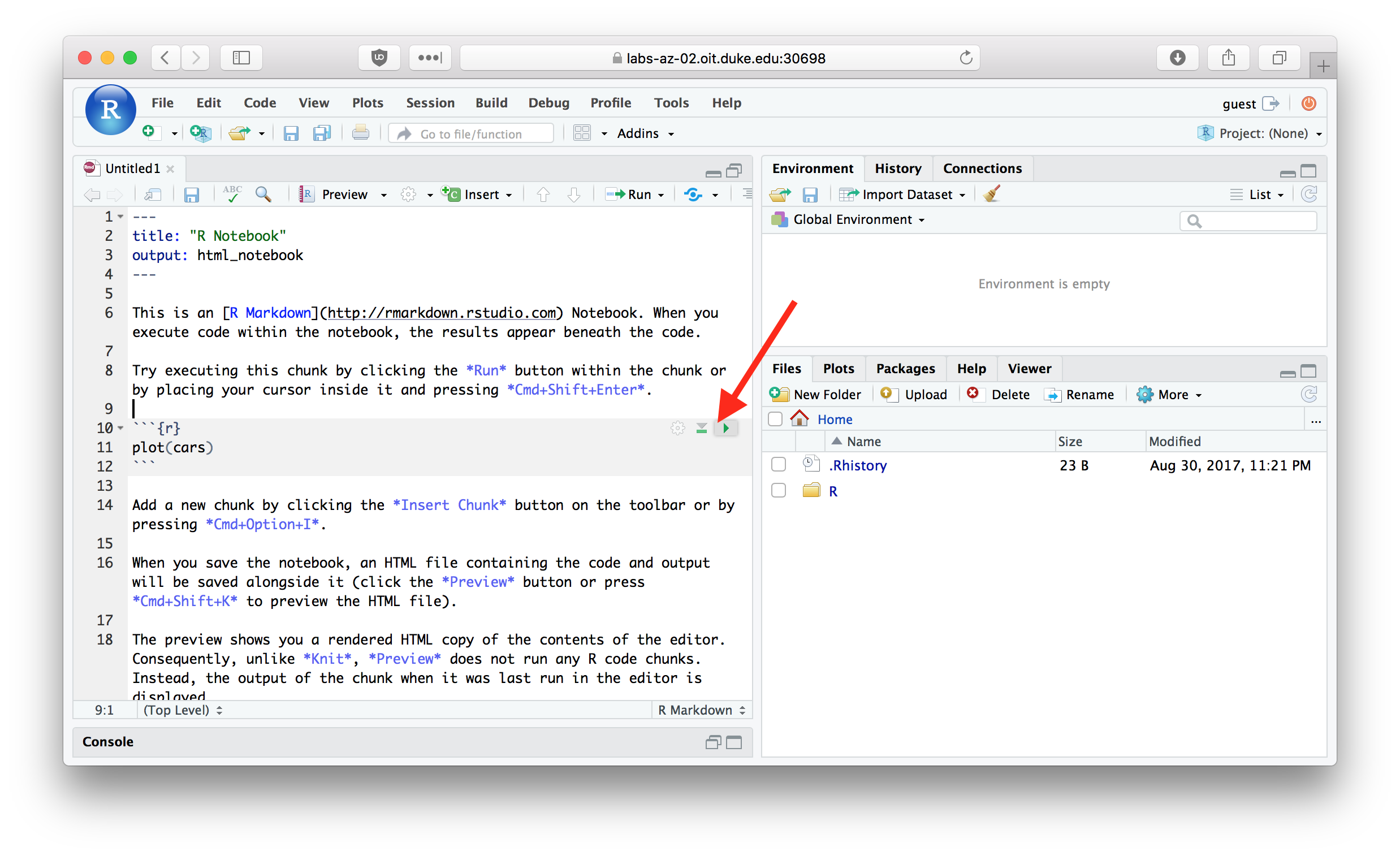
This is the default interface setup of Rstudio. Of course you can customize it, but this is what you should see out-of-the-box:

Below is a brief description of the purpose of each tab. The ones we will be using most frequently in this course are highlighted in bold.

1. In section A you will find the Console, Terminal, and Background Jobs tabs

   • Console: This is arguably the most important tab in Rstudio. It provides direct access to the R interpreter, allowing you to run code and see outputs.

     There are a few other useful tips for working in the console:

     • You can use the TAB key to autocomplete code as you type. This works both for built in functions, user-defined objects, or even file paths (more on this later).

     It is highly recommended to use TAB as often as you can, not because it can save you keystrokes, but because it helps avoid typos!

     • You can also easily rerun previously executed commands by either using the up ↑ and down ↓ arrow keys to navigate through your history, or even search your history by using CTRL+R or ⌘+R.

   • Terminal: This tab opens a terminal in your current working directory (more on this later). By default, this is a Git Bash terminal on Windows and a zsh terminal on Macs, but this can be easily changed in the Options menu.

   • Background Jobs: Rstudio may sometimes run certain operations as background jobs here. Alternatively, you can also run background R scripts here if you desire.

2. In section B we have the Environment, History, Connections, and Tutorial tabs
   • Environment: This is probably the second most important tab in Rstudio. Any created variables, defined functions, imported datasets, or other objects used in your current session will appear here, along with some brief descriptions about them.
     • The broomstick icon in this tab can be used to clear the current session environment, removing all defined objects. This is basically equivalent to restarting Rstudio.
     • Next to the broomstick, there’s an icon that shows the memory usage of your current R session, as well as an “Import Dataset” option that can help you load datasets, although we will primarily try to write this code by hand for learning purposes.
   • History: In this tab, you will find a history of previous commands from your current session, if you want to edit and rerun something. You can also search through this history, which will search through not just your current session but ALL previous commands anytime you opened Rstudio in the past.
   • Connections/Tutorial: You can start special data connections, or find some extra R tutorials here if you wish.
3. In section C are the Files, Plots, Packages, Help, Viewer, and Presentation tabs.
   • Files: This tab gives you a small, integrated file explorer. You can navigate around your computer, create/delete/rename files, copy/move files, etc.
   • Plots: Any plots/graphs you make will show up here (if you set the options right, otherwise they may show in a pop-up). There are a few other useful features to know:
     • In the top left corner of this tab, there are left/right arrows for navigating between previous and next plots (if you made multiple plots)
     • Next to that, there’s a “Zoom” button which opens the plot in a larger window.
     • Next, there’s an “Export” button which allows you to export the plot to image/pdf/clipboard. This opens a window with additional export options.
     • Next, there are buttons to remove the current plot, or clear all plots.
   • Packages: Here you can view/install/update/load/unload packages. Note you can also install packages using the console, like we did in the previous section.
   • Help: This is one of the other most useful tabs in Rstudio. Here, you can access the built in R help pages. This is one of the FIRST places you should visit for help with R functions/objects.
     • There are several ways to access the help pages. Suppose you want help with the install.packages() function. You can either run ?install.packages or help(install.packages) in the console, or put your cursor on the function in your code and hit the F1 key.
     • The help page may contain these following sections, each of which presents different types of information:
       1. Description, showing a brief summary of the purpose of the function
       2. Usage, listing available arguments (i.e. options). If an argument has an = sign and a value, this denotes the default value
       3. Arguments, where more details about the arguments can be found
       4. Details, where further details on the function can be found
       5. Value, which gives info on what the function returns as an output
       6. Sometimes, other sections may appear here with more specialized info
       7. At the end, you may also find some advanced notes, links to related functions, additional references, and example code demos.

       You should at least briefly scan the help page each time you encounter a new function. There are often several different ways to use a function depending on which/how arguments are set, and this can prevent you needing to “reinvent the wheel” by, for example, trying to manually change the output format when there’s already a built-in way to output to your desired format.

   • Viewer: This is where a preview of your Rmd document output will appear when knitting (which we learn very soon).
     • In the top corner, there are buttons letting you clear current or all viewer items, as well a button to open the viewer in a new window in your default web browser, which can also be useful sometimes for checking your work or printing/exporting.
   • Presentation: This final tab is useful if you ever make presentations in Rstudio, e.g. using R’s Beamer or reveal.js integrations.

That concludes the tour of the basic Rstudio interface. There is also a file editor window (also known as the source panel/window) which we will discuss later on, but for now, let’s learn to run some basic R commands!

2.3 Basics of R

In this section, we will give you a brief introduction to working with R. No prior coding experience is assumed. You are highly encouraged to copy and run the examples as you read. If you have time and capacity, you are also encouraged to peruse the linked help pages and extra reference links, but this is not mandatory.

2.3.1 Running R code

The main way to run R code is to type or copy into the console. Comments can be written after a hashtag # and will not be run. If there is output, it will be displayed either in the console directly if it’s text, or in the plot window if it’s visual. In these notes, output is shown in a separate box below, starting with ## .

Try running these examples below in your console and observe the output:

# this line is a comment and will not be run
# use the copy button in the top corner to easily run this example --->
print("output is shown here") # you can also add comments here

[1] "output is shown here"

The [1] that appears at the start of the output line just means this is the first output value. These bracketed numbers are not part of the actual output and should be ignored.

# a VERY simple barplot
# the c() function creates a vector of numbers
barplot(c(1, 3, 2))

All functions in these notes should automagically link to their online help pages (these are the same help pages inside Rstudio that we saw in the previous section). Try clicking on the barplot() function here or in the previous code block to see its help page.

2.3.2 Basic math

One of the first things you should learn about R is how to use it as a calculator to do basic math. Operators like +, -, *, /, ^, and parentheses ( ) work just like how you’d expect. Note R respects standard order of operations (see this page on operation order for more details).

(-5 * -3^2 + 4) / 7 - 6

[1] 1

R will sometimes output in scientific notation, especially if the number cannot be exactly numerically represented due to limitations of computers. For example, if you compute 2^50 R will show the result as 1.1259e+15, i.e. 1.1259×10¹⁵. You can also type in 1.1259e+15 and R will understand it as 1.1259×10¹⁵.

2^50

[1] 1.1259e+15

Also note due to limitations of how computers represent numbers, R often cannot distinguish between numbers that differ by less than about 10^-15, i.e. 0.000000000000001.³

You can also perform integer division in R, i.e. dividing to get the quotient and remainder, by using %/% for the quotient and %% for the remainder. This allows you to check, for example, if a number is even or odd.

13 %/% 2

[1] 6

13 %% 2

[1] 1

Operators like %/% or %% may seem strange at first, but they work just like any other binary operators in R such as + or ^ . There are other examples of such operators like %in% and %>% which we will learn about later.

Trigonometric functions sin(), cos(), tan(), (and their inverses asin(), acos(), atan() where the a– prefix means arc–), also work as you’d expect and use radian units. Note pi is conveniently predefined as \(\pi\). Hyperbolic trig functions also exist if you need them.

cos(2 * pi)

[1] 1

atan(-1) * 4

[1] -3.141593

Exponential and logarithm functions exp() and log(), also work as you’d expect and default to the natural base \(e\). Note the log function has an optional base argument for using a different base. There are also special base 10 and 2 versions log10() and log2() .

log(exp(2)) * log10(100)

[1] 4

log(3^5, base = 3)

[1] 5

Additionally, abs() computes the absolute value and sqrt() the square root (note by convention, ONLY the positive root is returned). Taking the square root of a negative number will return NaN.

sqrt(abs(-9))

[1] 3

2.3.3 Aside: function arguments

A quick aside about function “arguments” (i.e. additional options that can be set). In R, all arguments to functions have names (see each function’s help page for details) but depending on how the function is needed, you might not have to set them explicitly.

In the previous section, we used base = 3 inside the log() function to explicitly set the base argument as 3. However, log(3^5, 3) will also work, since base is the second argument (again, see the help page). Without explicit naming, arguments are passed in order to the function.

Explicitly naming an argument is often used to clarify for teaching purposes, improve debugging legibility, or skip certain preceding arguments that are either unnecessary or whose default values are acceptable. E.g. suppose a function f() has 3 arguments, a, b, and c in that order. If you only wish to set a=0 and c=1 while leaving b blank, you can write f(0, c=1).

2.3.4 Special values

We already mentioned pi is predefined. There are a few other important special values in R. TRUE and FALSE, along with their abbreviations T and F are also predefined. Note the capitalization; R is a case-sensitive language so true, True, and t are NOT the same as TRUE (the first two are not defined, while t() is the matrix transpose function).

T

[1] TRUE

true

Error: object 'true' not found

An important thing to note is that in R, doing any kind of math turns TRUE into 1 and FALSE into 0.

exp(FALSE) * (TRUE + sqrt(TRUE))

[1] 2

Mathematical expressions may also return NaN for Not a Number, i.e. undefined; or Inf for infinite. Note R differentiates between positive infinity Inf and negative infinity -Inf.

sqrt(-4)

[1] NaN

1 / 0

[1] Inf

log(0)

[1] -Inf

Additionally, NA is used to represent missing values, i.e. when data is not available. Note NA and NaN are NOT the same. We will learn later about how to handle NA missing values.

2.3.5 Assignment

In R, variables are typically assigned using the <- operator, which is just a less than < and minus - put together. You can also use = but <- is recommended for stylistic reasons (see this blog post for more details). For this class, both are acceptable but we will prefer <- in the notes.⁴

# this is preferred
x <- 5
print(x)

[1] 5

# this is equivalent and acceptable, but discouraged
x = 5
print(x)

[1] 5

You can quickly insert the assignment <- operator with ALT+- on Windows or ⌥+- on Mac.

Generally, = is reserved for setting arguments inside functions, e.g. like the previous code chunk where we computed log() with a custom base by setting the base argument.

log(3^5, base = 3)

[1] 5

Variable names can be any combination of upper and lower-case letters, numbers, or period . and underscore _ (which are both treated similar to letters), with one caveat: variables must begin with a letter or period, not a number or underscore. You may not use any other characters in variable names.⁵

# these variable names are ok,
# also remember R is case sensitive!
var1 <- 1
Var1 <- 2
.OtherVariable <- 3
another.variable_42 <- 4

var1 + Var1 + .OtherVariable + another.variable_42

[1] 10

# even these morse code looking variable names,
# while not recommended, are technically ok:
. <- 1
.. <- 2
._ <- 3
._..__ <- 4

. + .. + ._ + ._..__

[1] 10

# these variable names will raise errors:
#   1var, _var, bad-var,   e.g.:
1var <- 1

Error: unexpected symbol in "1var"

Observe that if the results of an expression are saved to a variable, R will NOT print it by default. This is often confusing to first time R users, since it may seem like nothing happened. For example, running the following:

result <- 3 * 4 - 5

produces no visible output. This is normal behavior, since the output has been redirected into a variable. To inspect the result, you must explicitly call or print() the object again:

result

[1] 7

2.3.6 Summary functions

So far, we’ve only seen functions that run on individual values, but there are also functions in R that run on and summarize a dataset. These are often statistical in nature. We will only give a brief summary here of how to compute these in R. A more in-depth discussion of their meaning and applications will be saved for later in the course.

Suppose we gather a sample and observe the following values: 3, 6, 6, 2, 4, 1, 5 (don’t worry about what these mean, we’re just using it as a demo). We can create a vector using the c() function to store our data and save it:

data <- c(3, 6, 6, 2, 4, 1, 5)
data

[1] 3 6 6 2 4 1 5

The sum() and length() functions work like you expect and produce the sum and length of the sample. You can use them to compute the mean of your sample, which can also be done directly using mean().

sum(data) / length(data)

[1] 3.857143

mean(data)

[1] 3.857143

We can also find the median (i.e. middle number) with the median() function. (Sadly, there’s no built-in mode function in R, but this can be achieved with other packages.)

median(data)

[1] 4

We can generalize from the median (which is the 50-th percentile) to compute any percentile using the quantile() function, e.g. suppose we want to compute the 30-th percentile:

quantile(data, 0.3)

30% 
2.8 

The standard deviation is another important statistic (think of it as the distance of the average observation from the mean) and can be computed using sd(). Note this is equivalent to the square root of the variance which can be found with var().

sqrt(var(data))

[1] 1.9518

sd(data)

[1] 1.9518

We can also find the min() and max() of the sample (which together give us the range() of the dataset).

min(data)

[1] 1

max(data)

[1] 6

Another important function for working with samples is the %in% operator, which lets us check if a value exists in the dataset.

# 6 appears in the sample
6 %in% data

[1] TRUE

# 7 does not appear in the sample
7 %in% data

[1] FALSE

One final statistical function that is extremely common is cor() which computes the correlation between 2 vectors. E.g. suppose you had the following \((x,y)\) points: (3.4,1), (5,4.6), (5.7,6.8), (6.5,5.3). You can compute the correlation between the \(x\) and \(y\) points like so:

x <- c(5, 6.5, 3.4, 5.7)
y <- c(4.6, 5.3, 1, 6.8)
cor(x, y)

[1] 0.8690548

There are other miscellaneous functions for working with vectors that are sometimes useful that we won’t cover in detail now, but you can explore them on your own, such as prod() for computing the product of all numbers in a vector, sort() for sorting a vector, rev() for reversing a vector, unique() for getting the unique values in a vector, scale() for linearly shifting and scaling the data to have mean 0 and standard deviation 1, and cumsum() and cumprod() for the cumulative sum and product along a vector, and many many more…

2.3.7 Logical comparison

Finally, let’s learn some basic logical comparisons. These will be crucial for data cleaning and filtering operations later on.

In R, equality comparison is done using the == operator. Note the double equal sign; single equal is for assignments and arguments. Inequality can be checked using !=.

x <- (2 + 3)^2
x == 25

[1] TRUE

# if instead we ask "is x not equal to 25", we should get FALSE
x != 25

[1] FALSE

Note ! used individually is the NOT operator, i.e. it turns TRUE into FALSE and vice versa.

!TRUE

[1] FALSE

# this is equivalent to x != 25
!(x == 25)

[1] FALSE

Inequalities are done using <, <=, >, >=, for less than (or equal to) and greater than (or equal to).

x < 30

[1] TRUE

x >= 25

[1] TRUE

Logical statements can be chained together using the & AND operator as well as the | OR operator (on most keyboards, this vertical bar character is typed using SHIFT+\).

& will only return true if the expressions on both sides are both true; | will return true if at least one of the expressions on both sides is true. Note that & appears higher on R’s order of operations than |.

(x > 20) & (x <= 30)

[1] TRUE

(x > 20) | (x != 25)

[1] TRUE

You can of course chain these together with other R commands to compare more complicated expressions. The sky is the limit!

# check if x² is even OR if mean of data + 2 * sd is greater than the max
# note order of operations means we don't need extra parentheses
# of course, you can add extra parentheses for readability if you wish!
x^2 %% 2 == 0 | mean(data) + 2 * sd(data) > max(data)

[1] TRUE

Since computers don’t have infinite precision, some arithmetic operations can introduce small errors, especially those producing repeating-decimal or irrational numbers:

1/2 + 1/3 == 5/6

[1] FALSE

1/2 + 1/3 - 5/6

[1] -1.110223e-16

sqrt(2)^2 == 2

[1] FALSE

sqrt(2)^2 - 2

[1] 4.440892e-16

These imprecisions usually result in errors of 10^-15 or less. Generally values around this magnitude in R should be treated as indistinguishable from 0. When comparing inexact values like these, it’s recommended to use all.equal() instead of ==, which allows for a small tolerance.

all.equal(1/2 + 1/3, 5/6)

[1] TRUE

all.equal(sqrt(2)^2, 2)

[1] TRUE

2.3.8 Packages

Now, let’s briefly discuss packages. One of the best features of R is the ability for anyone to easily write and distribute packages on CRAN (Comprehensive R Archive Network). Currently, there are 21788 packages available on CRAN. There are also a further 2289 packages on the bioinformatics-specific package archive Bioconductor, as well as countless more on GitHub.

In this course, we will primarily make use of the Tidyverse suite of packages, which contains several important packages for data science: readr for reading in data, ggplot2 for plotting data, dplyr and tidyr for cleaning data, and lubridate and stringr for working with dates and strings. We will learn each of these as the course progresses.

The most important thing you need to remember about packages is this:

install once; load daily

I.e. you only need to install a package once to your computer, but you need to load it every time you reopen Rstudio and want to use it (unless you’re one of those people that never closes any programs). Of course if you want to setup R/Rstudio on a new computer, you need to install it again there as well.

2.3.8.1 Install a package

Unless you’re doing extremely niche work, generally any packages you want to use will be on CRAN and can be easily installed one at a time by running the following.

# you should have already installed tidyverse from last chapter
# note the package name MUST be in quotes
install.packages("tidyverse")

It’s important to check the output messages to see if the install was successful, and if not, to find important “Error:…” keywords to use for troubleshooting. Sometimes R will ask you different things during install:

• If R asks you to use a “personal library”, say yes. This just means it can’t store the package files in your system directory due to system permissions, so it will store it somewhere else (typically in your user directory).
• If R asks you to install “from source”, try no first; if that fails, retry with yes. This just means if you want R to prioritize using precompiled executable files when installing, which is generally much faster.
• If R asks you to update existing packages before installing a new package, this is entirely up to you. I like to update my packages regularly, but there’s usually no harm if you don’t want update immediately.
  • If you try to update packages that are currently loaded, R may ask you to first “restart R”, which is usually a good idea.

2.3.8.2 Loading a package

You can load a package with either library() or require(), which are basically the same.⁶ Some package names actually load a group of other packages, e.g. library(tidyverse) will load all the “core” Tidyverse packages, which include ggplot2, dplyr, tidyr, readr, purrr, tibble, stringr, and forcats.

library(tidyverse)

── Attaching core tidyverse packages ────────────── tidyverse 2.0.0 ──
✔ dplyr     1.1.4     ✔ readr     2.1.5
✔ forcats   1.0.0     ✔ stringr   1.5.1
✔ ggplot2   3.5.1     ✔ tibble    3.2.1
✔ lubridate 1.9.3     ✔ tidyr     1.3.1
✔ purrr     1.0.2     
── Conflicts ──────────────────────────────── tidyverse_conflicts() ──
✖ dplyr::filter() masks stats::filter()
✖ dplyr::lag()    masks stats::lag()
ℹ Use the conflicted package (<http://conflicted.r-lib.org/>) to force all conflicts to become errors

Upon loading, many packages will print various diagnostic messages to the console. These are generally completely ignorable. Sometimes these will warn about “Conflicts”, this is standard and just means it has overridden other default functions. E.g. You can see above the filter() function from the package dplyr has overwritten the pre-loaded filter() function from the stats package.

You may have already guessed from the message in the output above, but you can also access a function from another package without loading the entire package by using the syntax package::function(). This is often done to either avoid name conflicts or to clarify to the reader which functions come from which packages.

2.3.9 Whitespace

As a final topic, let’s briefly discuss spacing. “Whitespace” refers to any sequence of space-type characters, which can be a mix of spaces, tabs, and line breaks (i.e. when you hit ENTER).

R ignores whitespace between variable names, functions, and punctuation characters. E.g. the following are all equivalent:

# these are all the same
mean(data)

[1] 3.857143

mean ( data )

[1] 3.857143

mean (
  data
)

[1] 3.857143

A long line of code is often broken across several lines for readability. We will see many examples of this shortly in the data visualization chapter.

However, make sure if you break a line up to finish the line eventually, otherwise you’ll get an error. For example, if you type mean(data in the console but forget to close the parenthesis (try this!) you will see the prompt character > be replaced with +. It will continue to do this, patiently waiting for you to finish the line, until you either close it by typing ) OR cancel the line by hitting ESC.

2.3.10 R cheat sheets

Those are probably the most important R commands you need to know for now. Below I have curated a short selection of R “cheat sheets” for your reference should you need it, in rough order of how useful I think it will be for a first time R learner.

• Matt Baggott’s R Reference Card v2.0 is a nice complete one-stop-shop for all of R’s built-in functions.
• IQSS’s Base R Cheat Sheet and Alexey Shipunov’s One Page R Reference Card are both slightly shorter and more curated, but offer a nice, tighter set of the most critical R commands, along with useful examples of their syntax.
• For a slightly longer but more complete reference manual on R, especially with more details of how R works and different object types and data structures, Emmanuel Paradis’s R for Beginners may be helpful.

2.4 R Markdown

In this next section, we will introduce you to R Markdown, which is a document format that allows you to seamlessly organize and integrate text and R code/output in an easily readable and editable way. It supports many output file types including HTML, PDF, and DOCX, and can be used to write reports, articles, presentations, ebooks, and even websites (in fact, this entire website is written in R Markdown, and the GitHub repo even maintained using Rstudio; you can view the source code of any page using the “View source” button in the right sidebar).

Let’s start with an example! Below is a basic R Markdown demo file called demo.Rmd, which produces demo.html as output. We will use this example below to learn how to work with Rmd files.

---
title: "Demo Rmd file"
author: "Jane Doe"
date: "2024-06-20"
output: html_document
---

```{r setup, include=FALSE}
# this is a standard "setup" chunk usually found at the top of Rmd files,
# often used for setting options, loading files, and importing libraries
knitr::opts_chunk$set(echo = TRUE)
library(tidyverse)
```

# Section 1

## Subsection A

Here's some ordinary text. You can use Markdown syntax to add more features, e.g. here's a [link](https://markdownguide.org/cheat-sheet), here's some **bold text**, and here's some `inline code`. You can also add images, footnotes, blockquotes, and more. See linked cheat sheet above for more.

 1. Lists are also east to add!
 2. Here's a second item.
 3. You can even add sublists:
    - Here's a sublist with bullets.
    - Another bullet?

## Subsection B

You can easily incorporate R code into an Rmd file, with outputs and plots that auto-update. Here's an example code chunk named "chunk1".

```{r example-chunk, fig.height=5, fig.align="center"}
data <- c(3, 6, 6, 2, 4, 1, 5)
mean(data)
hist(data)
```

You can even refer to R objects inside text, e.g. the sample mean and standard deviation are `r mean(data)` and `r sd(data)`.

# Section 2

Here's a second section.

<!-- comments in an Rmd file must use HTML-style syntax -->

2.4.1 Source window

Download the demo.Rmd example file and open it; it should automagically open in Rstudio in a new panel in the top left called the source window, which is actually just a basic text editor like Notepad or TextEdit, but with some additional R-aware features (more on this later).

2.4.2 Knitting

The first thing you should learn about R Markdown is how to “Knit”, or generate an output document. Think of an Rmd file as a “recipe” that tells Rstudio how to create and format a nice output for your audience.

At the top of the source window, find the Knit button and click it. You’ll see a bunch of messages scroll by in a new tab below called “Render” while Rstudio executes and processes the document. If there are no errors, Rstudio will then produce the output document “demo.html” in the same directory where you saved “demo.Rmd” and open a preview of the file in the “Viewer” tab.

You can also knit by pressing CTRL+SHIFT+K on Windows, and either CTRL+SHIFT+K, or ⌘+SHIFT+K on Mac.

If you do run into errors, look for a line with the keyword “Error: …”. Usually, searching this error message in your favorite search engine is a good way to diagnose the problem.

As we continue learning more about R Markdown below, feel free to play around with this demo Rmd file and re-knit to see the resulting changes.

2.4.3 YAML header

Rmd files usually start with a YAML header with some important metadata about the file:

---
title: "Demo Rmd file"
author: "Jane Doe"
date: "2024-06-20"
output: html_document
---

Title, author, and date are self explanatory. The output: option sets the output format R uses when knitting. We highly recommend using the default html_document output format since it is lightweight, portable, and easy for us to view in Canvas when grading.

There are lots of other YAML options you can explore, but minimally, you should always have these 4: title, author, date, and output: html_document set at the beginning of each Rmd document.

2.4.4 Markdown

R Markdown is based on Markdown⁷ which is a simple syntax for “marking up” text with additional formatting. You can see mixed in with paragraphs of ordinary text, there are # Section and ## Subsection headings, [links](url) and **bold text**, lists and sublists, and both inline and separate “chunks” of source code.

We will not expect you to learn ALL of markdown, but minimally you should learn to use section and subsection headings, links and lists, and both inline code and code chunks.

2.4.5 Code

There are two main ways to include code in an R Markdown file: inline and chunks.

2.4.5.1 Inline code

If you want to quote R code inside a paragraph of text, surround it with the backtick character `, which can be found on most keyboards in the top left next to the 1 key. Note this character is NOT the same as a single quote character ’. For example, this: `mean(data)` will render as: mean(data).

You can also easily refer to R variables and substitute their values, or apply other functions to them and display the output inside text. For example, remember how the data vector was defined above in section 2.3.6? This: `r median(data)` will render as: 4. Note the `r prefix here, which triggers evaluation and substitute of the code. This helps avoid “hard-coding”, letting values and references update to always stay in sync.

If a value has too many digits after the decimal, e.g. `r mean(data)` becomes: 3.8571429, it is highly recommended to round the result off to a reasonable number of digits using either round() or signif(). So in this case, `r round(mean(data),2)` which becomes 3.86 is much better.

It is also important to only round at the END, when you present your analysis. Do NOT round your original dataset or an intermediate value used in another computation, as this will introduce errors that can compound.

Generally, I recommend rounding to either the same precision as your data, or 2-3 significant figures; we will not be too picky about the exact number of digits. See this page for more discussion about precision and rounding.

2.4.5.2 Code chunks

The other prominent way to include R code inside an R Markdown document is by using so-called code “chunks” or “blocks”. The basic structure is this:

```{r example-chunk, fig.height=5, fig.align="center"}
data <- c(3, 6, 6, 2, 4, 1, 5)
mean(data)
hist(data)
```

You can quickly insert a chunk by using CTRL+ALT+I on Windows, and either CTRL+⌥+I, or ⌘+⌥+I on Mac.

A code chunk has this basic structure:

1. Chunks always start with ```{r where the r indicates this will contain R code to be executed.

2. This is then optionally followed by a space and a name for the chunk, e.g. example-chunk. While a name is not necessary, it is recommend for 2 reasons:

   1. If your code has errors and you name all your chunks, R will tell you the name of the chunk with the error, which can help you troubleshoot faster.
   2. R will also use chunk names (along with section headings) to generate a document outline at the bottom left of the source window. You can click on this outline button and quickly navigate to another part of a long Rmd file.

3. This name can also optionally be followed by a comma , followed by additional “chunk options”, which are extra settings you can set to control the behavior of the chunk and output. There is a VERY long list of available options, but here is a short list of some of the MOST important:

   Option	Possible values (default values in bold)	Description
   eval	TRUE, FALSE	Controls whether code in chunk is evaluated.
   echo	TRUE, FALSE	Controls whether code in chunk is echoed (i.e. displayed). Note code can be evaluated without echoed, echoed without evaluated, or both/neither.
   include	TRUE, FALSE	Setting this to FALSE will run the chunk, but hide both the code AND output. This is often used in a “setup chunk” near the top of a document to import packages, load datasets, and do other “setup tasks” that you want to hide.
   error	TRUE, FALSE	Controls whether to allow errors and continue knitting. Note this option is FALSE by default, meaning R will halt and not produce output if it encounters any errors.
   fig.width, fig.height	any number; default: 7, 5	These control the size of the plot output, if there is one.
   fig.align	“default”, “left”, “right”, “center”	This controls the alignment of the plot output, if there is one. Note this option MUST be set with quotes. “default” does not set an alignment.
   cache	TRUE, FALSE	If a chunk is time consuming, you can “cache” it. Cached chunks will not be rerun unless the code inside is modified. Note this is set FALSE by default. This option should be used with caution! Improper usage may cause code chunks to not update properly.8

   One last note: remember the “setup” chunk at the top of the demo file? Here it is again:

   ```{r setup, include=FALSE}
   # this is a standard "setup" chunk usually found at the top of Rmd files,
   # often used for setting options, loading files, and importing libraries
   knitr::opts_chunk$set(echo = TRUE)
   library(tidyverse)
   ```

   The function knitr::opts_chunk$set() here can be used to set default chunk options for ALL chunks in that document, e.g. you can center all figures by adding fig.align = "center" here instead of copying it to every chunk header.

4. After closing the header with } and starting a new line, you can now put whatever code you want inside the chunk. All code here gets run one line at a time and output displayed.

5. At the end, the chunk is closed by another set of ```.

Remember you can also use TAB autocomplete in Rmd code chunks to save keystrokes and avoid typos! You can even TAB autocomplete chunk options.

This concludes the discussion of code chunks in R Markdown.

2.4.6 Aside: \(\LaTeX\)

This is also outside the scope of this course, so you do NOT need to learn it, but R Markdown natively supports \(\LaTeX\) code as well. It’s rendered using MathJax, an open-source Javascript engine for rendering equations online. For example, $$x=\frac{-b\pm\sqrt{b^2-4ac}}{2a}$$ becomes:

\[x=\frac{-b\pm\sqrt{b^2-4ac}}{2a}\]

You will see lots of \(\LaTeX\) later in the notes when I need to write more math, so I just wanted to mention it here. You can right click on any equations you see in the notes and change the MathJax display options, or see its source code (you can of course also see the source code of the entire page using the link in the sidebar as mentioned previously).

If you wish to read more on \(\LaTeX\), start with Rong Zhuang’s MathJax cheat sheet or David Richeson’s quick guide which both have lots of great beginner-friendly examples. For a slightly more complete list of symbols, Eric Torrence’s cheat sheet may also be useful.

2.4.7 Cheat sheet

If you need a good R Markdown cheat sheet, I recommend this reference guide published by the same developers as Rstudio. Page 1 has a Markdown syntax guide, pages 2-3 highlight some more useful chunk options, and pages 4-5 have some additional info on different output formats as well as some additional YAML header options.

2.5 Workflow

In this final section, we will briefly discuss some workflow considerations for working with Rstudio and R Markdown that are important to know for troubleshooting purposes.

2.5.1 Working directory

The “working directory” is a concept first-time R users always struggle with. Simply put, R always runs as if it’s inside a directory. The current directory R is running from inside of is called the “working directory”. You can check your current working directory with the getwd() function:

# check current working directory
getwd()

[1] "/home/admin/stat240-revamp"

You can see my current Rstudio session (while writing these notes) is running from the stat240-revamp directory which is itself located in /home/admin.

Generally, when you start a new Rstudio session, the working directory will default to C:/Users/username/ for Windows and /Users/username/ for Mac (or /home/username/ for Linux, which the server building these notes each day runs), where username is your account name (my working directory is different because I have it intentionally set to my notes project folder).

This default working directory actually presents a problem, because it is usually different from where your current Rmd file is. For example, suppose you’re working on homework 1. If you organized your files properly—which you should!—your Rmd file is probably located at .../STAT240/homework/hw01/hw01.Rmd. For reasons explained in the next section, your working directory should always match the location of your current Rmd file.

You can do this by either of these methods:

• Recommended: Using the top menu bar, go to “Session” > “Set Working Directory” > “To Source File Location”. This sets the working directory to where the location of the current file being edited.
  • For Windows users, the shortcut for this is ALT+S, then release both keys and type W and S one at a time.
  • For both Windows and Mac, you can also setup a custom shortcut for this action. From the top menu bar, go to “Tools” > “Modify Keyboard Shortcuts…”, find “Set Working Directory to Current Document’s Directory” and set your preferred shortcut. Mine is set to CTRL+SHIFT+D but feel free to choose your own.
• You can also set it automagically to your current Rmd file location with try(setwd(dirname(rstudioapi::getSourceEditorContext()$path)),silent=T) which can be run either in the console, or copied into any Rmd file (e.g. in the setup chunk) and run whenever you open the file.
• You can also set it manually by running setwd() in the console if you prefer.

Whenever you open Rstudio, OR switch to a different file, you should ALWAYS do the following:

1. Set your working directory,
2. Load any necessary packages,
3. Read in any necessary datasets.

2.5.2 Knitting v. console execution

But why do we need to match the working directory to our Rmd file location? This is where the difference between knitting and execution comes into play.

It turns out, code runs differently in an Rstudio console than when being knit in an Rmd file. Code in the console will always run in your current working directory, and any objects created will be added to your current session Environment. They will stay there until you clear the Environment.

However, when you Knit a document, it will create a new R session in the background with the working directory set to the same location as the Rmd file, and run the entire document from scratch, top to bottom and then produce an output file. This means if your working directory in Rstudio is not set to the same place, it can break file references if you need to load any datasets.

This may seem overly complicated right now, but it will quickly become intuitive as you practice more.

2.5.3 Tips

Before I end this chapter, I want to offer a few tips for your workflow that I find myself repeating over and over to nearly every student, especially when errors arise.

1. The MOST important tip for avoiding/fixing errors is knit often, and check the output! Why?
   • Knitting is the best way to catch errors, and the more often you knit, the easier it will be to identify the source of the error (since there’s less new code to check).
   • Knitting will automatically save your document for you, helping avoid lost work due to crashes.
   • You can check the formatting of new document elements, whether they are bodies of text, markdown features, plot outputs, code, etc..
   • If you run into unexpected computer or Rstudio problems, you’ll have a more recently-knit output you can submit in the interim while you troubleshoot.
2. Another tip is in general, think of Rstudio’s console as a place to “test out” a new line of code you’re trying to add. Continue to test it until you’re satisfied with it, then immediately copy it into your Rmd. Work that you do in the console is NOT saved! Your Rmd file is where all your work is saved and then knit into a final output.
   • You can easily run a line of code in an Rmd file in the console by putting your cursor anywhere on that line and using CTRL+ENTER on Windows and either CTRL+ENTER or ⌘+ENTER on Mac. To run an entire chunk, add SHIFT to the previous shortcut combo. You can also use the top-right chunk shortcut buttons.
3. Remember knitting always creates a NEW, empty background R session, sets the working directory to the Rmd file location, then runs the entire file top to bottom. This means:
   • If you run a line in the console without copying it into the Rmd file, that line will NOT be run when you knit.
   • If you define an object in the console, forgot to copy it into the Rmd file, then try to use it somewhere else in the file, you WILL get an error.
   • Objects must be defined BEFORE they are used in an Rmd file. If you define data on line 20 but try computing mean(data) on line 10, you WILL get an error.⁹
   • If your working directory does not match the location of your current Rmd file, this may also cause errors if you need to load any datasets. Remember to always set your working directory!
4. You have an error? Have you tried the following?
   1. Read the error message! Look for “Error:…” and read it or search it in a browser! If you’re knitting, there should also be a line number or chunk name (remember to name your chunks!) that should help you find where the problem code is.
   2. Check you’re using the function correctly. Read the built-in help page for the function, or search online for some example usages.
   3. Check if your input object (this is often the output from an earlier line or chunk) is actually correct. E.g. if data wasn’t properly created in chunk-1, it might not show an error until you try to compute mean(data) in chunk-2 below. Be paranoid! Check each input and output as you go along!
   4. If you imported lots of packages, check if your function names have conflicts. E.g. if both package1 and package2 have a function func1, you may accidentally be using the wrong one. You can check this by also opening the help page for func1 and checking to see which help page it directs to.
   5. If you still can’t identify the problem, restart your R session by going to the top menu bar > “Session” > “Restart R”, then run your entire Rmd ONE function at a time, checking EACH function’s output along the way. This may take longer, but will almost always work.
   6. If you tried everything and STILL can’t figure it out, ask us for help.

Phew, that was a lot, but that wraps up the introduction to working with R/Rstudio! Below, I have linked a few bonus readings if you want to learn a bit more about control and looping in R, which we will not need in this class but may be good to know if you plan to take further data science classes or build a career in data science.

In the next chapter, we will explore data types and structures in R, as well as learn to read in and write out datasets.

Optional bonus topic: control/looping

This includes if/else statements and for/while loops. If you’re interested, see these suggested readings:

• This page by Yihui Xie from the bookdown documentation offers a good & quick overview of control and looping in R.
• For a more in-depth discussion, check out this page by Hadley Wickham from his Advanced R book.